Approved by COSEWIC in April 2009
Area of Occupancy is a biological measure of the occupied habitat within a wildlife species’ range. When estimated at a scale that is biologically relevant to a wildlife species, area of occupancy can provide insights into the wildlife species habitat requirements, threats and limitations, and, if data are available over time, valuable trend information. This is important biological information that is relevant to assessment criteria and as contextual information for assessment. It is important to keep in mind that COSEWIC uses area of occupancy in two ways. First, it uses it in a very specific way in the form of an index tied to thresholds in the quantitative criteria. For clarity this treatment of area of occupancy is referred to as Index of Area of Occupancy or IAO. Area of Occupancy is also used in its more general sense as a biological defensible estimate of the occupied habitat within a wildlife species’ range. Note that in the latter case, this information cannot be used within the quantitative criteria but can be important to the overall assessment. This information is to be used as a contextual consideration as part of assessment step 4, or in step 5, where the results of the assessment are evaluated against the definitions of the assessment categories (COSEWIC Status Assessment and Designation).
Index of Area of Occupancy (IAO) is used by COSEWIC as part of Criteria B and D. The size of COSEWIC’s IAO for a wildlife species is compared against threshold values in the COSEWIC criteria to identify wildlife species with a restricted distribution or small population size and thereby wildlife species which may have an elevated risk of extirpation or extinction. Because the estimated size of IAO is dependent on the scale at which it is measured, it is important to use a consistent scale when determining IAO for use in the COSEWIC criteria. COSEWIC has determined that an IAO measured at a scale of 2x2 km² (or, sometimes, 1x1 km² as detailed below) is appropriate for use with the criteria.
The COSEWIC guidelines for calculating and reporting IAO are provided in Part A, below. These recommendations were accepted by COSEWIC in November 2006 based on analyses provided by the Criteria Working Group of COSEWIC.
A. COSEWIC guidelines for calculating and reporting IAO
1. COSEWIC will adopt a 2x2 km grid for the calculation of IAO, as a matter of routine, so that the criterion thresholds for IAO can be applied in a consistent and meaningful manner.
2. A 1x1 km grid may be used if (a) enough data are available and (b) the smaller grid is justified (e.g. a very specific habitat requirement such as freshwater or sand dunes). Refer to IUCN section 4.10.6 for caveats regarding use of a 1x1 grid for “linear” habitats.
Both the 2x2 and 1x1 IAO should be reported so that they can be compared with one another and against the thresholds. The rationale for the recommended use of the 1x1 must be provided in the status report. It is up to the COSEWIC membership to determine which of the two estimates are most appropriate for assessment.
Note that IAO is never used in isolation when applying the quantitative criteria; there is always some other indicator of risk of extinction that must be met, such as decline rate, severe fragmentation, few locations, threats etc.
3. Area of occupancy information other than IAO estimates may also be relevant to a status assessment and inclusion of this information in the status report is encouraged. When Area of Occupancy rather than IAO is estimated this must be biologically defensible, that is enough data and information must be available, including where the wildlife species occurs and does not occur, that an accurate estimate of occupied habitat can be made. These estimates cannot be used in combination with the grid-size dependent thresholds. Estimates of Area of Occupancy are to be discussed in relation to the affect on extinction risk as part of the consideration of contextual considerations in step 4 of the assessment or in step 5 where the results of criteria and guideline application are compared with the definitions of the assessment categories (see COSEWIC Status Assessment and Designation).
B. COSEWIC process for calculating IAO
As indicated in the Instructions to Status Report Authors, report authors must contact the Secretariat regarding calculation of IAO. SCC Co-chairs are also encouraged to contact the Secretariat if they require assistance or have questions with IAO. If questions cannot be resolved please refer them to the Criteria Working Group.
C. Guidance: IUCN guidelines for IAO and Area of Occupancy
Information and guidance on the use of IAO can be found in Section 4.10 of Guidelines for Using the IUCN Red List Categories and Criteria and is provided below.
Note that there is some confusion in this document regarding area of occupancy in general and the grid-method used in the criteria context. For the most part the IUCN use of AOO is the same as COSEWIC IAO.
Area of Occupancy (AOO) is a parameter that represents the area of suitable habitat currently occupied by the taxon. As any area measure, AOO requires a particular scale. In this case, the scale is determined by the thresholds in the criteria, i.e. valid use of the criteria requires that AOO is estimated at scales that relate to the thresholds in the criteria. These scales (see “Problems of scale” below) are intended to result in comparable threat status across taxa; other scales may be more appropriate for other uses. For example, much smaller scales are appropriate for planning conservation action for plants, and larger scales may be appropriate for global gap analysis for large mobile wildlife species. However, such scales may not be appropriate for use with the criteria.
Area of Occupancy is included in the criteria for two main reasons. The first is to identify wildlife species with restricted spatial distribution and, thus usually with restricted habitat. These wildlife species are often habitat specialists. Wildlife species with a restricted habitat are considered to have an increased risk of extinction. Secondly, in many cases, AOO can be a useful proxy for population size, because there is generally a positive correlation between AOO and population size. The veracity of this relationship for any one wildlife species depends on variation in its population density.
Suppose two wildlife species have the same EOO, but different values for AOO, perhaps because one has more specialized habitat requirements. For example, two wildlife species may be distributed across the same desert (hence EOO is the same), but one is wide ranging throughout (large AOO) while the other is restricted to oases (small AOO). The wildlife species with the smaller AOO may have a higher risk of extinction because threats to its restricted habitat (e.g. degradation of oases) are likely to reduce its habitat more rapidly to an area that cannot support a viable population. The wildlife species with the smaller AOO is also likely to have a smaller population size than the one with a larger AOO, and hence is likely to have higher extinction risks for that reason.
4.10.1 Problems of scale
Classifications based on the area of occupancy (AOO) may be complicated by problems of spatial scale. There is a logical conflict between having fixed range thresholds [in the criteria] and the necessity of measuring range at different scales for different taxa. “The finer the scale at which the distributions or habitats of taxa are mapped, the smaller the area will be that they are found to occupy, and the less likely it will be that range estimates … exceed the thresholds specified in the criteria. Mapping at finer spatial scales reveals more areas in which the taxon is unrecorded. Conversely, coarse-scale mapping reveals fewer unoccupied areas, resulting in range estimates that are more likely to exceed the thresholds for the threatened categories. The choice of scale at which AOO is estimated may thus, itself, influence the outcome of Red List assessments and could be a source of inconsistency and bias.” (IUCN 2001) Some estimates of AOO may require standardization to an appropriate reference scale to reduce such bias. Below, we first discuss a simple method of estimating AOO, then we make recommendations about the appropriate reference scale, and finally we describe a method of standardization for cases where the available data are not at the reference scale.
4.10.2 Methods for estimating AOO
There are several ways of estimating AOO, but for the purpose of these guidelines we assume estimates have been obtained by counting the number of occupied cells in a uniform grid that covers the entire range of a taxon (see Figure 2 in IUCN 2001), and then tallying the total area of all occupied cells:
AOO = no. occupied cells × area of an individual cell (equation 4.1)
The ‘scale’ of AOO estimates can then be represented by the area of an individual cell in the grid (or alternatively the length of a cell, but here we use area). There are other ways of representing AOO, for example, by mapping and calculating the area of polygons that contain all occupied habitat. The scale of such estimates may be represented by the area of the smallest mapped polygon (or the length of the shortest polygon segment), but these alternatives are not recommended.
4.10.3 The appropriate scale
It is impossible to provide any strict but general rules for mapping taxa or habitats; the most appropriate scale will depend on the taxon in question, and the origin and comprehensiveness of the distribution data. However, we believe that in many cases a grid size of 2 km (a cell area of 4 km²) is an appropriate scale. Scales of 3.2 km grid size or coarser (larger) are inappropriate because they do not allow any taxa to be listed as Critically Endangered (where the threshold AOO under criterion B is 10 km²). Scales of 1 km grid size or smaller tend to list more taxa at higher threat categories than these categories imply. However, if the available data were obtained as the result of high-intensity sampling, these finer scales may be appropriate. In other words, in order to use a finer scale of, say, 1 km grid size, the assessors should be reasonably certain that empty 1-km² cells represent real “absences” rather than “undetected presences”. For most other cases, we recommend a scale of 4 km² cells as the reference scale. If an estimate was made at a different scale, especially if data at different scales were used in assessing wildlife species in the same taxonomic group, this may result in inconsistencies and bias. In any case, the scale for AOO should not be based on EOO (or other measures of range area), because AOO and EOO measure different factors affecting extinction risk (see above). If AOO can be calculated at the reference scale of 4 km² cells, you can skip sections 4.10.4 and 4.10.5. If AOO cannot be calculated at the reference scale (e.g., because it has already been calculated at another scale and original maps are not available), then the methods described in the following two sections may be helpful.
4.10.4 Scale-area relationships
We recommended reducing the biases caused by use of range estimates made at different scales by standardizing estimates to a reference scale that is appropriate to the thresholds in the criteria. This and the following section discuss the scale-area relationship that forms the background for these standardization methods, and describe such a method with examples. The method of standardization depends on how AOO is estimated. In the following discussion, we assume that AOO was estimated using the grid method summarised above. The standardization or correction method we will discuss below relies on the relationship of scale to area, in other words, how the estimated AOO changes as the scale or resolution changes. Estimates of AOO may be calculated at different scales by starting with mapped locations at the finest spatial resolution available, and successively doubling the dimensions of grid cells. The relationship between the area occupied and the scale at which it was estimated may be represented on a graph known as an area-area curve (e.g., Figure. 4.3). The slopes of these curves may vary between theoretical bounds, depending on the extent of grid saturation. A maximum slope = 1 is achieved when there is only one occupied fine-scale grid cell in the landscape (fully unsaturated distribution). A minimum slope = 0 is achieved when all fine-scale grid cells are occupied (fully saturated distribution).
| grid length | grid area | AOO |
|---|---|---|
| 1 | 1 | 10 |
| 2 | 4 | 24 |
| 4 | 16 | 48 |
| 8 | 64 | 64 |
| 16 | 256 | 256 |
| 32 | 1024 | 1024 |
Celebrating 100 years of bird conservation
History, migratory birds convention, bird caring tips.
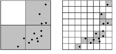
Figure 4.3. Illustration of scale-dependence when calculating area of occupancy. At a fine scale (map on right) AOO = 10 x 1 = 10 units2. At a coarse scale (map on left) AOO = 3 x 16 = 48 units2. AOO may be calculated at various scales by successively doubling grid dimensions from estimates at the finest available scale (see Table). These may be displayed on an area-area curve (above).
4.10.5 Scale correction factors
Estimates of AOO may be standardized by applying a scale-correction factor. Scale-area relationships (e.g,. Figure. 4.3) provide important guidance for such standardization. It is not possible to give a single scale-correction factor that is suitable for all cases because different taxa have different scale-area relationships. Furthermore, a suitable correction factor needs to take into account a reference scale (e.g., 2 km grid size) that is appropriate to the area of occupancy thresholds in criterion B. The example below shows how estimates of AOO made at fine and coarse scales may be scaled up and down, respectively, to the reference scale to obtain an estimate that may be assessed against the AOO thresholds in Criterion B.
Example: Scaling Up
Assume that estimates of AOO are available at 1km grid resolution shown in Figure. 4.3 (right) and that it is necessary to obtain an estimate at the reference scale represented by a 2 km grid. This may done cartographically by simply doubling the original grid dimensions, counting the number of occupied cells and applying equation 4.1. When the reference scale is not a geometric multiple of the scale of the original estimate, it is necessary to calculate an area-area curve, as shown in Figure. 4.3, and interpolate an estimate of AOO at the reference scale. This can be done mathematically by calculating a scale correction factor (C) from the slope of the area-area curve as follows:
C=( log 10 ( AOO 2 / AOO 1 ) log 10 ( Ag 2 / Ag 1 )) (equation 4.2)
Where AOO1 is the estimated area occupied from grids of area Ag1, a size close to, but smaller than the reference scale, and AOO2 is the estimated area occupied from grids of area Ag2, a size close to, but larger than the reference scale. An estimate of AOOR at the reference scale, AgR, may thus be calculated by rearranging equation 2 as follows:
AOO R = AOO 1 * 10 C*log( Ag R /Ag 1 ) (equation 4.3)
In the example shown in Figure 4.3, estimates of AOO from 1x1 km and 4x4 km grids may be used to verify the estimate AOO at the reference scale of 2x2 km from the as follows:
C=( log 10 (48/10)/log(16/1))=0.566, and
AOO=48* 10 0.566*log(4/16) =22 km 2
Note that this estimate differs slightly from the true value obtained from grid counting and equation 1 (24km2) because the slope of the area-area curve is not exactly constant between the measurement scales of 1x1 km and 4x4 km.
Example: Scaling Down
Scaling down estimates of AOO is more difficult than scaling up because there is no quantitative information about grid occupancy at scales finer than the reference scale. Scaling therefore requires extrapolation, rather than interpolation of the area-area curve. Kunin (1998) and He and Gaston (2000) suggest mathematical methods for this. A simple approach is to apply equation 4.3 using an approximated value of C.
An approximation of C may be derived by calculating it at coarser scales, as suggested by Kunin (1998). For example, to estimate AOO at 2x2 km when the finest resolution of available data is at 4x4 km, we could calculate C from estimates at 4x4 km and 8x8 km as follows.
C=(log(64/48)/log(64/16))=0.208
However, this approach assumes that the slope of the area-area curve is constant, which is unlikely to hold for many taxa across a moderate range of scales. In this case, AOO at 4x4 km is overestimated because C was underestimated.
AOO=48* 10 0.208*log(4/16) =36 km 2
While mathematical extrapolation may give some guidance in estimating C, there may be qualitative information about the dispersal ability, habitat specificity and landscape patterns that could also provide guidance. Table 4.1 gives some guidance on how these factors may influence the values of C within the range of scales between 2x2 km and 10x10 km grid sizes.
| Biological characteristic | Influence on C | |
|---|---|---|
| Small (approaching 0) | large (approaching 1) | |
| Dispersal ability | Wide | localised or sessile |
| Habitat specificity | Broad | Narrow |
| Habitat availability | Extensive | Limited |
For example, if the organism under consideration was a wide-ranging animal without specialized habitat requirements in an extensive and relatively uniform landscape (eg., a species of camel in desert), its distribution at fine scale would be relatively saturated and the value of C would be close to zero. In contrast, organisms that are either sessile or wide ranging but have specialized habitat requirements that only exist in small patches within the landscape (e.g., migratory sea birds that only breed on certain types of cliffs on certain types of islands) would have very unsaturated distributions represented by values of C close to one. Qualitative biological knowledge about organisms and mathematical relationships derived from coarse-scale data may thus both be useful for estimating a value of C that may be applied in equation 4.3 to estimate AOO at the reference scale.
Finally, it is important to note that if unscaled estimates of AOO at scales larger than the reference value are used directly to assess a taxon against thresholds in criterion B, then the assessment is assuming that the distribution is fully saturated at the reference scale (i.e., assumes C = 0). In other words, the occupied coarse-scale grids are assumed to contain no unsuitable or unoccupied habitat that could be detected in grids of the reference size.
4.10.6 "Linear" habitat
There is a concern that grids do not have much ecological meaning for taxa living in "linear" habitat such as in rivers or along coastlines. Although this concern is valid, for the purpose of assessing taxa against criterion B, it is important to have a measurement system that is consistent with the thresholds, and that leads to comparable listings. If AOO estimates were based on estimates of length x breadth of habitat, there may be very few taxa that exceed the VU threshold for Criterion B (especially when the habitats concerned are streams or beaches a few metres wide). In addition, there is the problem of defining what a "linear" habitat is, and measuring the length of a jagged line. Thus, we recommend that the methods described above for estimating AOO should be used for taxa in all types of habitat distribution, including taxa with linear ranges living in rivers or along coastlines.
4.10.7 AOO based on habitat maps and models
Habitat maps show the distribution of suitable habitat for a wildlife species. They may be derived from interpretation of remote imagery and/or analyses of spatial environmental data using simple combinations of GIS data layers, or by more formal statistical habitat models (e.g. generalised linear and additive models, decision trees, Bayesian models, regression trees, etc.). Habitat maps can provide a basis for estimating AOO and EOO and, if maps are available for different points in time, rates of change can be estimated. They cannot be used directly to estimate a taxon’s AOO because they map an area that is larger than the occupied habitat (i.e. they also map areas of suitable habitat that may presently be unoccupied). However, they may be a useful means of estimating AOO indirectly, provided the three following conditions are met.
i) Maps must be justified as accurate representations of the habitat requirements of the wildlife species and validated by a means that is independent of the data used to construct them.
ii) The mapped area of suitable habitat must be interpreted to produce an estimate of the area of occupied habitat.
iii) The estimated area of occupied habitat derived from the map must be scaled to the grid size that is appropriate for AOO of the wildlife species.
Habitat maps can vary widely in quality and accuracy (condition i). A map may not be an accurate representation of habitat if key variables are omitted from the underlying model. For example, a map would over-estimate the habitat of a forest-dependent montane species if it identified all forest areas as suitable habitat, irrespective of altitude. The spatial resolution of habitat resources also affects how well maps can represent suitable habitat. For example, specialised nest sites for birds, such as a particular configuration of undergrowth or trees with hollows of a particular size, do not lend themselves to mapping at coarse scales. Any application of habitat maps to Red List assessment, should therefore be subject to an appraisal of mapping limitations, which should lead to an understanding of whether the maps over-estimate or under-estimate the area of suitable habitat.
Habitat maps may accurately reflect the suitable habitat, but only a fraction of suitable habitat may be occupied (condition ii). Low habitat occupancy may result because other factors are limiting - such as availability of prey, impacts of predators, competitors or disturbance, dispersal limitations, etc. In such cases, the area of mapped habitat could be substantially larger than AOO and will therefore need to be adjusted (using an estimate of the proportion of habitat occupied) to produce a valid estimate of AOO. This may be done by random sampling of suitable habitat grid cells, which would require multiple iterations to obtain a stable mean value of AOO. Habitat maps are produced at a resolution determined by the input data layers (satellite images, digital elevation models, climate surfaces, etc.). Often these will be at finer scales than those required to estimate AOO (condition iii), and consequently scaling up will be required.
In those cases where AOO is less than the area of suitable habitat, the population may be declining within the habitat, but the habitat may show no indication of change. Hence this method could be both inaccurate and non-precautionary for estimating reductions in population change.
However, if a decline in mapped habitat area is observed (and the map is a reasonable representation of suitable habitat - condition i), then the population is likely to be declining at least at that rate. This is a robust generalisation because even the loss of unoccupied habitat can reduce population viability. Thus, if estimates of AOO are not available, then the observed decline in mapped habitat area can be used to invoke "continuing decline" in criteria B and C, and the rate of such decline can be used as a basis for calculating a lower bound for population reduction under Criterion A.